Reference manual for QRI's Oscilleditor
System requirements
The Oscilleditor is designed to be used on a computer. It will probably not work well, or at all, on a smartphone or tablet. But if there's enough interest, we might make a mobile-friendly version.
The Oscilleditor uses a technology called WebGL2 (with two extensions called EXT_color_buffer_float and OES_texture_float_linear) which are not supported on every computer. Specifically, support depends on the graphics card hardware in your computer, the graphics card driver software, and the web browser you use. Sadly we can't provide a list of all models that work or doesn't work - there are too many possible combinations. It has worked on all 10 computers we've tested on before release.
One of the 3 effects in the Oscilleditor (the "Coupled Oscillators" effect) can be quite demanding in terms of computing power. Specifically, the demand increases as you increase the coupling kernel radius, which forces the graphics card to read more and more pixels. If your computer is struggling to keep up, the Frames per Second counter will make that clear. If your computer is struggling but you want a large coupling kernel radius, there is another way to decrease the demand - increase the resolution halvings.
Data flow - the 3 effect types
The Oscilleditor has 3 main types of effects: Pattern Recognition, Coupled Oscillators, and Drifting. This diagram shows how they interact.
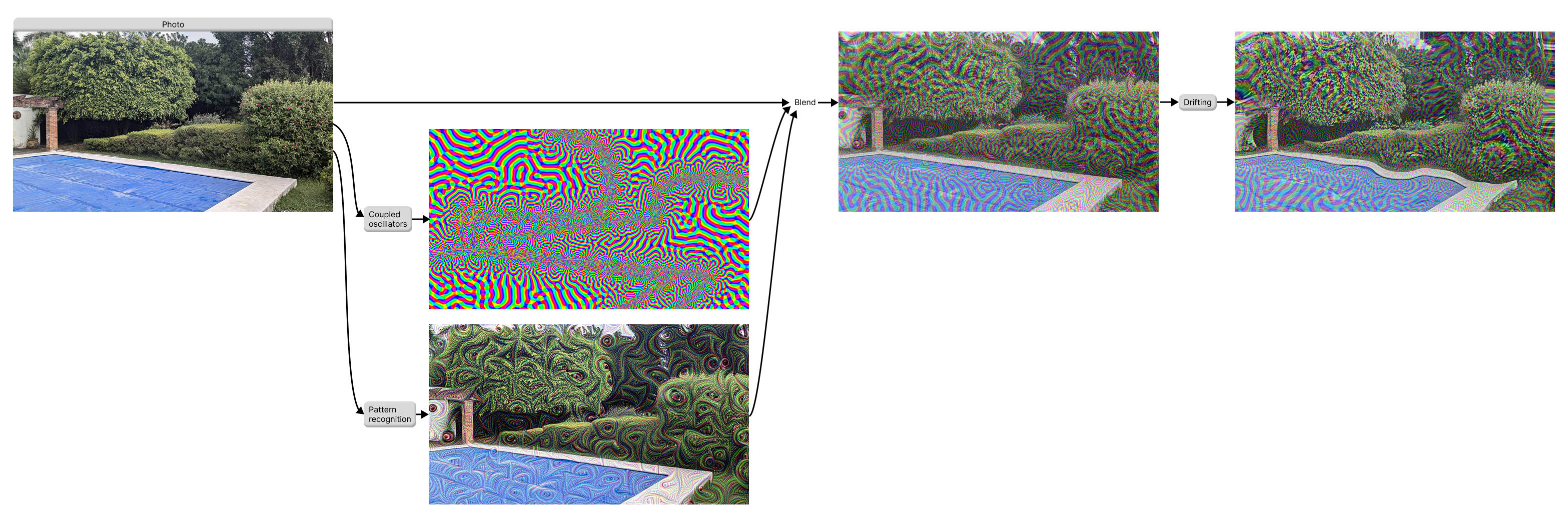
For the pattern recognition effect, we input the source photo into a neural network. The resulting images are stored permanently together with the original photos. In other words, this was a one-time job, the neural network doesn't run all the time.
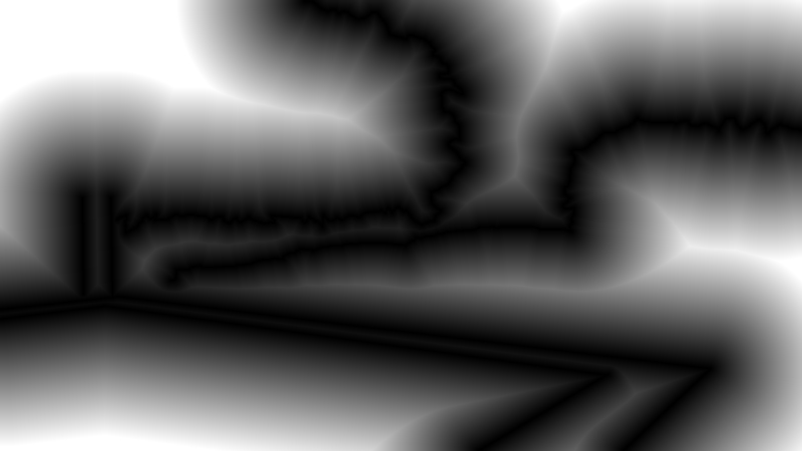
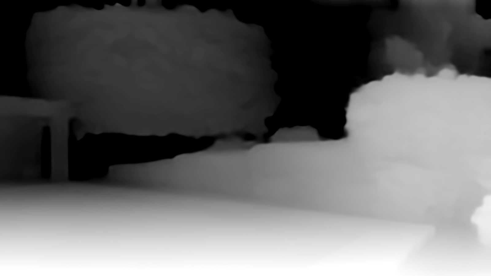
How is the photo an input to the Coupled Oscillators? It depends on what you choose in the GUI. The photo can affect two things: coupling kernel size, and oscillator natural frequency. Either from the photo brightness, depth, or edges (distance to nearest edge).
The original photo is then color blended with the oscillator output and the InceptionV3 output. How much you see of one effect or the other can be controlled by the two "opacity" parameters under Pattern Recognition and Coupled Oscillators Simulation, respectively.
Finally, this blended image is made to wobble by the Drifting effect.
GUI layout overview, main control buttons
Initially, the simulation is paused - you just see a still image. Underneath the image, there are buttons to control this, similar to any video player. Press the Play button to start running the simulation.
If the simulation is already paused, the Pause button is disabled. And vice versa, if the simulation is already playing, the Play button is disabled.
The "Single Step" button advances the simulation one frame forward in time.
Frames per second
Depending on your computer and your parameters, this simulation might be a very heavy task, which your computer might struggle with. After running for 1 second, the "Speed" display will update, it will say something like "60 fps". If it says something much lower, like for example "Speed: 10 fps", it means your computer isn't powerful enough to run the simulation at a smooth speed. If you want to increase the speed, either decrease the coupling kernel radius or increase Resolution Halvings.
Video recording
If you want to save a set of parameters, one way to do so is to record a video clip of the oscilleditor in action. (Another way is to export parameters.) There is a built-in video recording feature. Press "Record video" to begin recording. If the simulation was paused, it will also automatically start to play now. You will see a status message appear, saying something like for example "Recorded 1 sec, 1.22 MiB", which will update every second to show how the video grows in size. Then, press "Finish & download" which will stop recording, and pop up a save dialog so you can permanently save the recording to a file on your disk. The file is called oscilleditor_session.zip and if you open it, it contains video.webm and some other stuff.
The video compression algorithm used gives acceptable quality but unfortunately at quite large file sizes. If you want the best possible quality and/or smaller file sizes, we recommend you do a screen recording with a separate tool.
Presets
A list of parameter combinations that QRI found interesting, to serve as inspiration or starting points for your own exploration. If you select a preset and click "Load", this will change all the simulation parameters except the photo.
Photo selection
Press "Select Photo" to try a different background picture than the default one. This opens a "Choose a Photo" box. The oscilleditor includes 8 photos showing a variety of shapes, textures, natural and manmade scenery. Click one of the 8 small photo thumnails to start using it.
Or supply your own image. Note that this doesn't upload your image to any server on the internet, your image stays locally on your computer. You can choose an image with the Browse button, or you can drag&drop an image file from somewhere else on your computer into the box, or copy an image from anywhere and paste it (Ctrl+V or Cmd+V) while the "Choose a Photo" box is open.
Limitations: when you use your own image, there are no "DeepDream layers", so that part of the Pattern Recognition effect doesn't work. Also there is no "depth map", so the options "Kernel Shrinks By Depth" and "Frequencies Vary By Depth" don't work.
Drifting
The Drifting effect is a post-processing step applied after all other effects have been combined. It warps the final image by moving pixels around in a smooth, continuous way. You can think of it as placing the image on the surface of water, with waves.
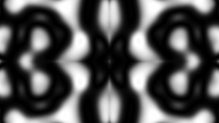
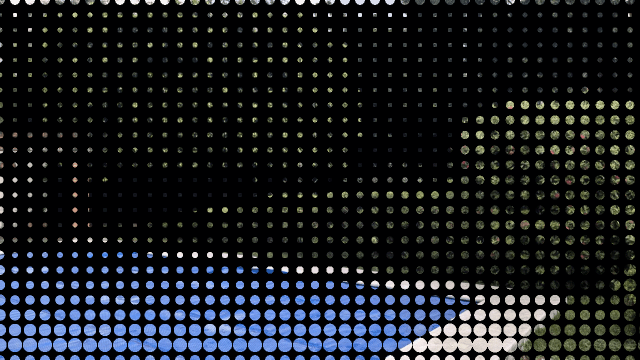
Just like the Coupled Oscillators simulation, drifting also is fundamentally an oscillating (wavy) effect. We could have run another full simulation for the driftning, but we don't, to save computing power. Instead, we recorded a short video loop of oscillators, blurred it a lot, and use that video to control the driftning. Here is the video loop:
Amplitude
Controls how far pixels are displaced from their original positions. All the displacement happens along a single direction, bottom-left to top-right. At zero, the image is completely static. As you increase the amplitude, the image appears to wobble and flow more strongly. The exact amplitude number is the maximum displacement as a fraction of the whole image, so for example if amplitude is 0.01, the max horizontal displacement is 1% of the image width, and max vertical is 1% of the image height.
Speed
Controls how fast the drifting pattern evolves over time, were 1 is the "normal" video playback speed.
Pattern Size
Controls the spatial scale of the drifting pattern. Small values create fine-grained, local distortions like frosted glass, while large values create broad, smooth movements affecting large regions of the image at once. The number is the width of the video in pixels. If this width is set to be smaller than the 1280*720 box that all effects happen inside, the drifting pattern is repeated. When we made the pattern, we didn't make it seamlessly tile-able, so to make the seams less jarring we use "mirrored" tiling.
Pattern Recognition
A common effect of psychedelics is an increase in a person's tendency to recognize patterns, for example eyes or faces, within vague stimuli. The Oscilleditor doesn't break any radical new ground here, but we include pattern-recognition effects for completeness.
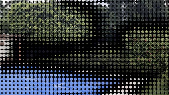
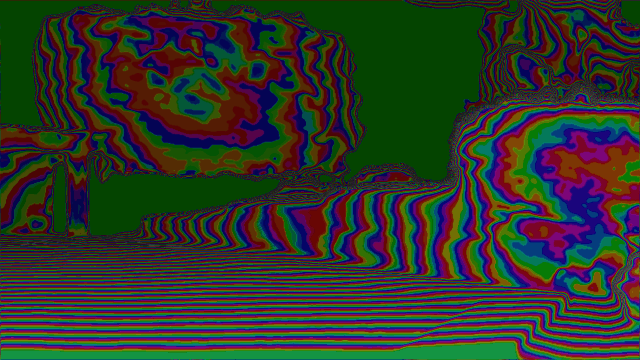
Similarly to in our Drifting effect, there is a short prerecorded video loop which controls where the pattern-recognition effect gets displayed or hidden. Below, we call it the "Mask". The mask grayscale value controls how the effect fades in and out in different locations on screen. Here is the video loop:
DeepDream Layer
Each photo comes with a set of 6 images which emulates the pattern-recognition effect. These images were pregenerated offline by a neural network, namely Google's InceptionV3. Use this dropdown selectbox to select one of the images aka layers. Lower layers emphasize simple aspects of the original photos. Higher layers show more complex patterns.
Use Video Pattern
This checkbox hides the DeepDream layer, which is a static picture, and replaces it with a trippy video loop.
Video Speed
How fast should the video pattern play? 1.0 is "normal" speed, here you can make it faster or slower.
Opacity
Opacity controls how the original photo and the pattern-recognition effect (the DeepDream layer or video) are mixed together, as a fraction between 0 and 1, where 0 means that the pattern is completely invisible. 1 means that they are shown at full strength. Note that even at full strength, the pattern isn't shown everywhere, only in some areas, due to the Mask.
Saturation
If you set saturation to 0, the pattern will only affect the brightness of the original photo. If you set it higher, the pattern will also affect the color hue, so the displayed photo might get more green in some places and more pink in other places, for example. The scale and the upper limit here is arbitrary.
Mask Speed
Controls how fast the mask evolves over time, were 1 is the "normal" video playback speed.
Mask Size
Controls the spatial scale of the mask. The number is the width of the video in pixels. If this width is set to be smaller than the 1280*720 box that all effects happen inside, the drifting pattern is repeated. It's designed to tile seamlessly.
Coupled Oscillators Simulation
This is the most complex effect in the Oscilleditor, with a lot of parameters. The effect runs on a square grid with the same size as the photo, 1280 * 720 pixels. Each pixel is a Kuramoto oscillator which, depending on parameters described further down, wants to synchronize or anti-synchronize with other nearby oscillators.
Opacity
Opacity controls how the original photo and the oscillator effect are mixed together, as a fraction between 0 and 1, where 0 means that the oscillators are completely invisible. 1 means that they take over and completely hide the underlying photo.
Colors
Since each pixel is fundamentally a Kuramoto oscillator, which spins through 360 degrees, how should its current angle be visualized on the screen? This dropdown lets you choose between a bunch of coloring schemes - they decide how an angle maps to a color.
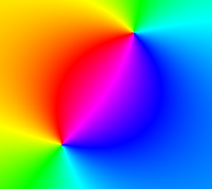
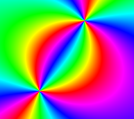
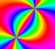
"Rainbow" simply maps each angle to a hue around the color wheel, so that 0 degrees is pure red, 60 is pure yellow, 120 is pure green, and so on up to 359 degrees.
"Black & white smooth, normal blending" maps the angle to a grayscale gradient between black and white, so 0 is white and 180 is black. "Normal blending" means that if you have two layers of oscillators, the final color is a weighted average of the colors from the two layers.
"Black & white smooth, interference blending" - same colors, but with a different way to blend between two layers of oscillators. It's not really related to wave interference, we should choose a better name.
"Black & white sharp, interference blending" - no grayscale gradient, just black and white like 60's op art. The final color is white if exactly one of the layers is white, but not if both of them are. In computer programming this is known as the "XOR" or "exclusive or" operation.
"Complementary colors sharp, normal blending" maps the angle (in oscillator layer 1) to a color gradient between blue at 0 degrees and yellow at 359 degrees, then immediately after yellow we jump straight back to blue, so the gradient is one-directional, it doesn't go back and forth. But in oscillator layer 2, the color gradient instead goes from green to magenta.
"Complementary colors sine, asymmetric" - the angle from layer 2 maps to a gradient between two complementary colors on opposite sides of the color wheel. The angle from layer 1 moves that layer 2 gradient partway around the color wheel - wobbles it back and forth between 23 and 157 degrees. So this is an asymmetric effect - the two layers don't work the same way.
"Complementary colors rotate, asymmetric" - the angle from layer 2 maps to a gradient between two complementary colors on opposite sides of the color wheel. The angle from layer 1 rotates that gradient all around the color wheel. So this is an asymmetric effect - the two layers don't work the same way. In this mode, the blending balance parameter has no effect.
Color windings
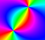
Packs color variation more tightly into the same space. For example, with "Rainbow" colors and windings set to 2, you will see with two full rainbows in one single oscillation. In other words, 0 and 180 degrees are both red, and X+180 is the same color as X. And with windings set to 3, the pattern repeats 3 times in one lap, and so on. The same logic applies to all color schemes including the black&white ones. Like all color settings, this is a purely visual effect that doesn't affect the underlying simulation.
Num layers
You can have 1 or 2 "layers" of oscillator simulation running in parallel. By default, the two layers are independent and don't affect each other, but you can make them affect each other with the cross-layer coupling parameter, which can give rise to very complex patterns. If you just have 1 layer, all the controls relating to layer 2 will be disabled.
Blending Balance
If you have two layers of oscillators, this controls how they get blended together. When the slider is close to 1, that layer is most visible. Around 1.5, both layers are equally visible. And when the slider is close to 2, that layer is most visible.
Layer 1 and Layer 2
Each of the two layers has an identical set of controls. If Num Layers is set to 1, all the controls relating to layer 2 will be disabled.
Log-Polar Transform
This checkbox can be on or off. When off, the oscillators run on a standard square grid, aka cartesian plane. When on, we switch to a log-polar coordinate system, which essentially measures distances from the origin (center of image) and angle to the origin. This feature is inspired by previous research about the mapping from the retina to the early visual cortex, and can be used to generate so-called "form constants" like cobwebs and flowers.
To be precise, our distance mapping is \frac{\ln(0.2 + distance \cdot 23)}{\pi}, where distance is not measured in pixels but in a different unit, scaled uniformly so the grid is 1 unit high and 1.7777... units wide (because the grid aspect ratio is always 16:9). So distance can vary between 0 (in the center of the image) and \sqrt(0.5^2+0.888^2) = 1.02 (at a corner of the image). The constants are somewhat arbitrary but have been tweaked to find the best compromise between two opposing goals: have the result stay mostly within the range 0-1, and minimize distortion near the center (where a plain log function would go towards negative infinity).
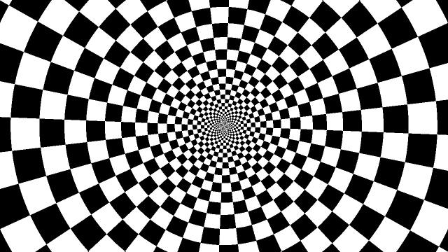
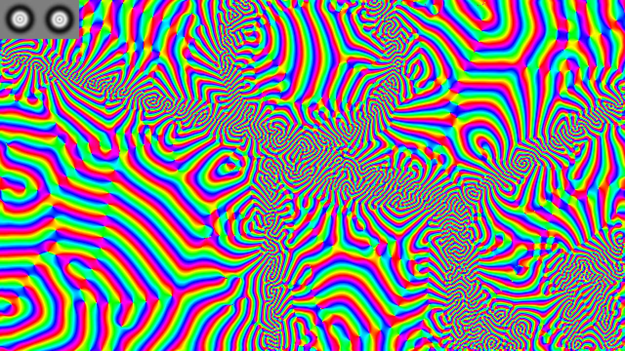
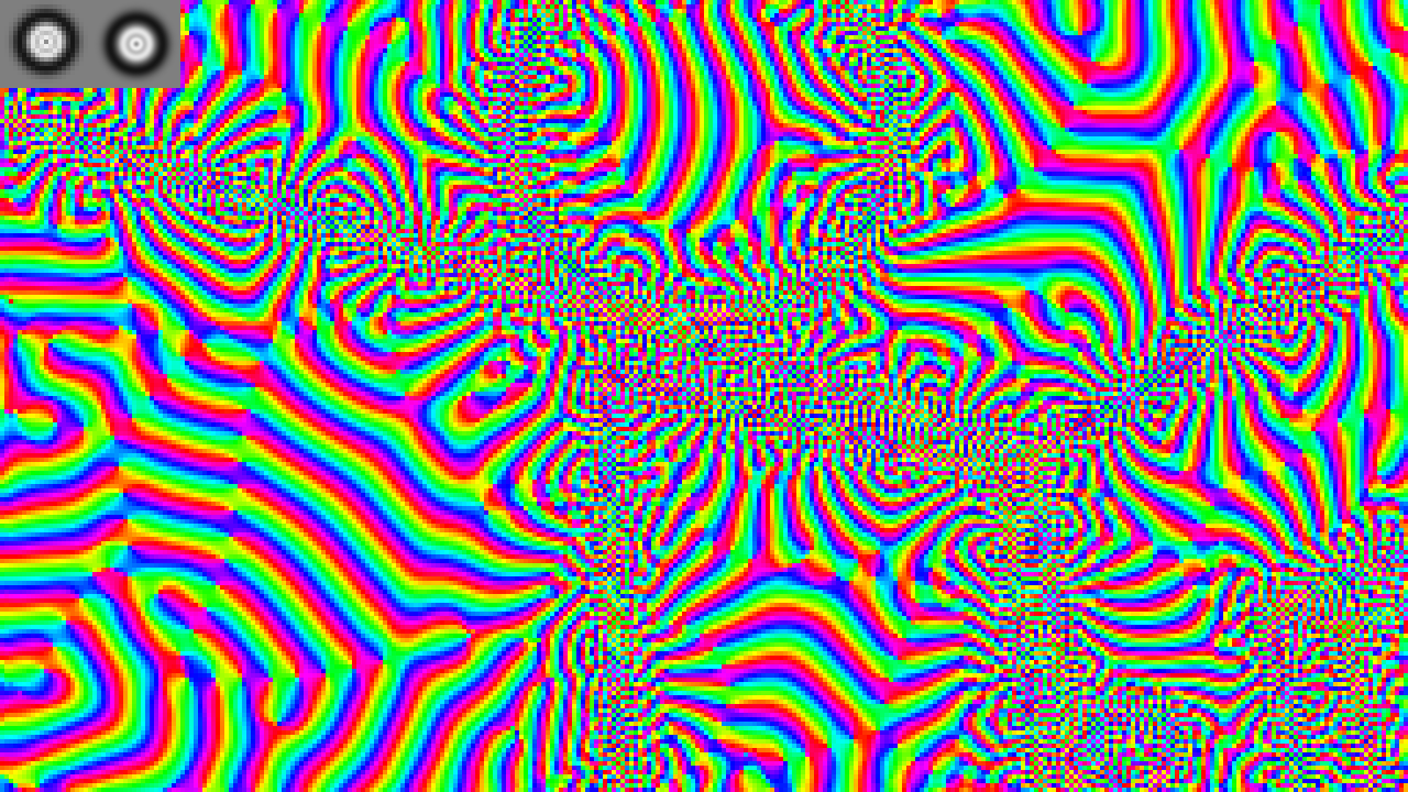
Resolution Halvings
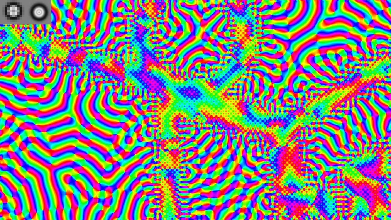
This feature was created as a way to increase simulation speed on weaker computers with large kernel radius. As described above, the simulation runs on a 1280 * 720 pixel grid. If your kernel radius is 10, that means the kernel has a diameter of 20, and the whole kernel is a 20*20 square. So for each pixel in the grid, we also read 400 neighboring pixels that the kernel covers, for a total of 1280 * 720 * 20 * 20 = over 368 million texture reads. This is true when "resolution halvings" is 0. But if we increase it to 1, the grid resolution gets halved in both x and y. And if we increase halvings to 2, the resolution gets halved again, and so on. Every halving in x and y reduces the number of pixels to one fourth, which saves a lot of computing power. The main disadvantage is that the image simulation gets blockier, until a pixel is bigger than the coupling kernel (or the kernel is smaller than a pixel, depending on how you think about it). The following pictures illustrate the logic of what happens. They are not directly representative of what you will see inside the actual tool.
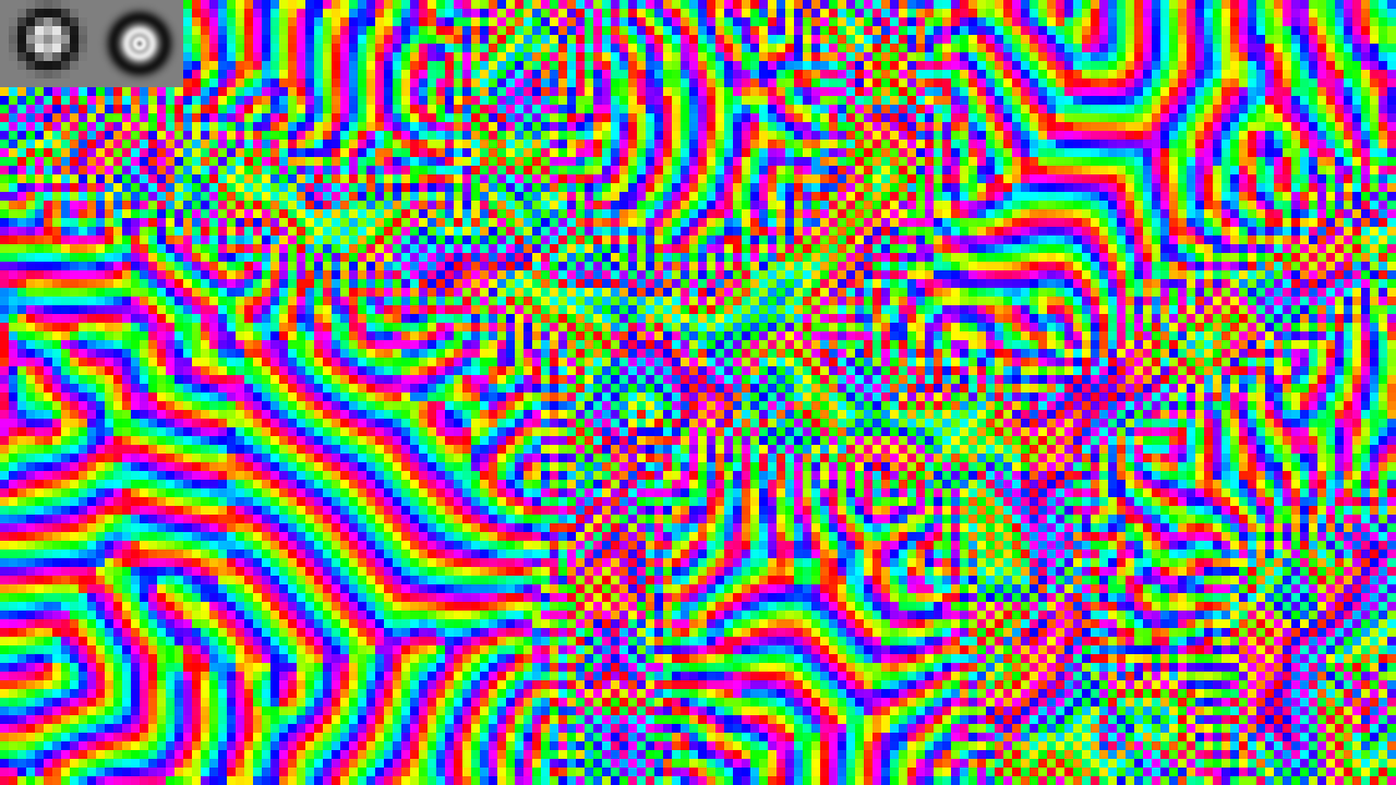
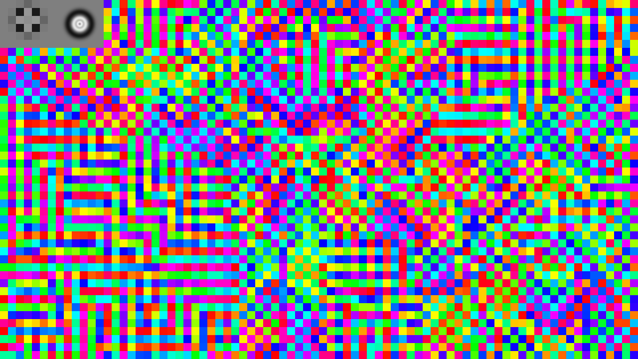
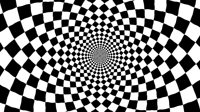
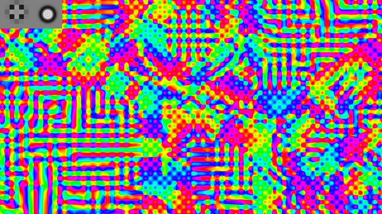
In practice, in the tool, the patterns will look less blocky even with Resolution Halvings > 0, because we smooth them out before display. So this is what 3 and 4 actually look like:
Kernel Radius
This scales the whole coupling kernel uniformly. It sets the outer radius in pixels of the kernel. (The distance numbers in the "Coupling kernel shape controls" table are relative fractions of this outer radius.) Specifically, it sets the maximum radius. Because the kernel can be smaller in some parts of the image, if you choose to set that option under Kernel Shrinks By, and the Kernel Shrink Factor number is a relative fraction of this maximum radius.
As you change the Kernel Radius, the grayscale preview in the top-left corner will resize in real time to show you how big the kernel is visually. If the simulation is playing, this preview will disappear automatically after 2 seconds. If the simulation is paused, this preview will disappear next time you change any other parameter that's not related to the kernel, or next time you Play or Single Step or so.
Kernel Shrinks By
By default, the kernel is the same size all over the image. But if you change this option, the kernel size can vary depending on the local image content, leading to interesting effects. Many people report that psychedelic patterns tend to emenate from edges or get attracted by edges, so therefore "kernel shrinks by edges" is one of our options. The other is "by depth". As you change this option, we illustrate what it will do with differently-scaled circles on the image.
If the simulation is playing, this preview will disappear automatically after 2 seconds. If the simulation is paused, this preview will disappear next time you change any other parameter that's not related to the kernel scaling, or next time you Play or Single Step or so.
The preview might mislead you to believe that the kernel is only applied at a few pixels in the grid, only where the circles are shown. But actully, the kernel is applied at every pixel in the grid, so we can't show every circle because they are overlapping. We just show a non-overlapping subset of circles as a limited but hopefully helpful illustration.
So as you see, we are providing the simulation with depth and edges as input. Obviously, the brain itself doesn't do that, it finds edges on its own and derives depth based on several clues. As we develop more sophisticated models in the future, we hope to make these effects emerge naturally out of the model itself.
Kernel Shrink Factor
Controls how much the kernel should change radius based on the shrinks by option. Fraction between 0 and 1, where 1 means it doesn't shrink at all. 0.5 means that exactly on an edge, where the kernel wants to shrink maximally, it will shrink to 50% of its max radius.
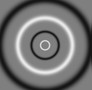
Coupling kernel shape controls
Our coupling kernel consists of 4 concentric rings.
This table of controls might look daunting to understand.
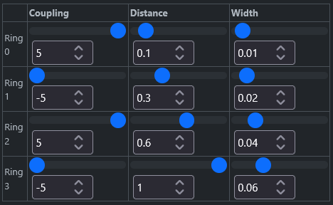
The controls allow you to control each of the 4 rings individually. "Distance" moves each ring in or out from the center, so 0 is exactly at the center, and 1 is all the way at the edge. You'll want to avoid having a ring all the way at the edge, because it will get abruptly clipped there, leading to artifacts in the simulation. If you want a larger ring, scale up the whole kernel with the kernel radius parameter.
"Width" makes each ring wider or narrower. Note that wider also means smoother, and narrower also means sharper.
Finally the most important value, "Coupling", decides what each ring means. A coupling number above 0 means that each oscillator will try to synchronize its oscillations with its neighbors that touch the ring, if we put the whole kernel centered on the oscillator in question. This positive coupling is displayed as white color in the diagram. The value also controls the strength of the coupling - the higher the number, the more I'll care about synchronizing with those neighbors. Coupling 0 means neutral, nothing in particular happens, which is displayed with gray. And below 0 means negative coupling, so each oscillator will try to anti-synchronize with its neighbors that touch the ring. This means they try to be maximally out of phase - if my neighbors are 10 degrees ahead of me, I'll slow down to try to make them 180 degrees ahead of me.
If you put one white and one black ring on top of each other, with the same width, they cancel out.
Mathematically, the kernel is defined as
- I(d) is the amount of influence that the neighbor has. Displayed as a color between black and white above.
- e is a constant: the base of the natural logarithm, approximately 2.718
- d is the distance from the neighbor to the "current" oscillator in the center of all the rings. This is the only variable. The rest are parameters rather than variables:
- C_i is the coupling strength of the i-th ring (controlled by "Coupling" sliders in the table)
- r_i is the radius of the i-th ring (controlled by "Distance" sliders in the table)
- w_i is the thickness of the i-th ring (controlled by "Width" sliders in the table)
As you change these coupling controls, the grayscale preview in the top-left corner will update in real time. If the simulation is playing, this preview will disappear automatically after 2 seconds. If the simulation is paused, this preview will disappear next time you change any other parameter that's not related to the kernel, or next time you Play or Single Step or so.
You might wonder what happens near the edges and corners of the simulation grid - how do we handle it when the kernel extends outside the grid? We use coordinate "wraparound" like in early videogames, so when the kernel extends above the top edge of the grid, we instead sample near the bottom edge. Topologically, that means the grid forms a torus / donut shape. We're not claiming that's what happens in the brain, it's just a convenient way to solve the problem in the simulation.
Coupling to Layer 2 / to Layer 1
If you have Num Layers = 2, by default the two layers are independent and don't affect each other, but you can make them affect each other with this parameter. This is a coupling number just like for the 4 rings above, so above 0 means positive coupling and so on. It will make each oscillator in one layer want to synchronize with the oscillator at the exact same place in the other layer.
Oscillator Frequencies
Each pixel - each Kuramoto oscillator - has its own frequency (its so-called "natural frequency"). If there was no influence from neighbors, it would simply always oscillate at its natural frequency. This section lets you control what those frequencies should be. In other words, imagine that each oscillator is like a hand on an analog clock, attached at the center of a circle, and gradually spinning around at some speed - this section controls how fast it wants to spin.
Min & Max
Sets the frequency, in Hz (oscillations per second) of the slowest and fastest oscillator. So what makes some oscillators slower and others faster? That's controlled by the next setting, "Frequencies Vary By".
Frequencies Vary By
"Depth" - uses the same depth map as in the Kernel Shrinks By setting. Oscillate at frequency proportional to the depth, the distance from the camera to the pixel. The pixels farthest away (black color) will oscillate at the "Min" frequency, and the pixels at the nearest possible depth (white color) will oscillate at the "Max" frequency. Note that this is holds even if you set min bigger than max. This option is disabled when you're using your own custom image.
"Edges" - uses the same edge distance map as in the Kernel Shrinks By setting. Oscillate at frequency proportional to the distance to the nearest edge. The pixels exactly at an edge will oscillate at the "Max" frequency, and the ones more than 255 pixels away from the nearest edge will oscillate at the "Min" frequency. Note that this is holds even if you set min bigger than max.
"Brightness" - Oscillate at frequency proportional to the pixel brightness. Black pixels will oscillate at the "Min" frequency, white pixels at the "Max" frequency. Note that this is holds even if you set min bigger than max.
"Grid Pattern" - generates a square-ish pattern of dots (hills and valleys alternating in a checkerboard pattern) of a given size. The "Size" slider controls the desired diameter (in pixels) of a 2x2 dot cluster. Why 2x2? Because one hill + one valley = 2 dots = one whole "wavelength". But you don't get exactly the desired diameter, because we round up or down it to fit an integer number of dots in the grid both horizontally and vertically. Why? So that the pattern wraps around seamlessly.
"Random noise" - each pixel oscillates at a frequency picked at random between Min and Max.
As you change the Min, Max, or "Frequencies Vary By" settings, the normal simulation graphics will be replaced with an illustration of the oscillator frequencies, to show you the logic of what's happening. Then after 2 seconds, the normal simulation graphics will automatically come back.
Phase reset buttons
These buttons, when clicked, change the phase of the oscillators. Imagine that each oscillator is like a hand on an analog clock, attached at the center of a circle, and gradually spinning around. While the "frequencies" section above controls how fast each hand spins, obviously each hand has a current position, and these buttons change that current position. And why would you want to do this? It's useful to explore how your chosen parameters behave when given a fresh start. Otherwise, since the field of oscillators has a kind of "memory", you couldn't know if the patterns you are seeing are completely determined by the current parameters, or if they are remains from some parameters you used a few seconds or minutes ago.
"Randomize phases" - When you click this button, each oscillator gets a random phase, somewhere between 0 and 359 degrees.
"Unify" - All oscillators get set to the same phase, 0 degrees.
"Plane waves H" - Creates so-called plane waves, a stripe pattern that will travel horizontally ("H") across the screen. All oscillators in a vertical column of pixels get set to the same phase, and the next column gets the next phase value, and so on. The wavelength is 32 pixels, we haven't made it configurable (yet). If you combine this with the log-polar transform, you get lines radiating out from the center.
"Plane waves V" - Same, but the waves travel vertically across the screen instead. If you combine this with the log-polar transform, you get concentric circles.
"Plane waves 45°" - Same, but with waves that travel diagonally instead. If you combine this with the log-polar transform, you get curved lines spiraling out from the center.
"Randomize All Phases" - just like "Randomize phases" but acts on both layer 1 and 2 at the same time.
"Unify All Phases" - just like "Unify" but acts on both layer 1 and 2 at the same time.
Export / import parameters
If you have found an interesting set of parameters that you want to save for later or share with other people, click "Share / export parameters". This will pop up a smaller window with the parameters exported in two different ways: URL and JSON.
If you have some JSON from the above, and want to use it, click "Import parameters".
If you have found an interesting set of parameters that reminds you of an experience you've had, please share it with Qualia Research Institute by clicking "Submit parameters" and fill out the form.